人工智能
使用 Amazon SageMaker HyperPod Data Capture 构建模型改进飞轮部署在 Amazon SageMaker HyperPod 上的基础模型会遇到任何预先整理的数据集都无法覆盖的输入:特定领域的行话、意料之外的格式、新产品以及不断变化的用户行为。如果没有生产推理数据的记录,团队就无法检测漂移、发现故障模式,也无法利用真实交互来改进模型。
Amazon SageMaker HyperPod 现在提供 Data Capture,这是一项内置能力,可在三个独立层级将实时推理输入和输出记录到 Amazon Simple Storage Service(Amazon S3),对延迟的影响极小,并且对模型可用性零影响。
在本文中,我们在单个 SageMaker HyperPod 集群上完整演示一个示例。一个家电客服路由模型捕获其生产流量,Amazon Athena 查询揭示出一个新产品盲点,一条 SQL 策略为捕获的记录打上标签,基于这些数据进行微调让该路由模型学会识别新产品。我们在模型部署前不可能存在的数据上,测量微调前后的准确率。推理算子在一个节点上提供模型服务,训练算子在另一个节点上运行微调。
本演练使用合成数据。脚本、清单、SQL、合成数据集和预期输出均可在 配套的 GitHub 仓库.
三层 Data Capture 架构
HyperPod Data Capture 提供三个独立层级,每个层级位于请求路径中的不同位置。你可以在同一个 dataCapture 块中开启任意组合。
| 层级 1:SageMaker 端点 | 层级 2:负载均衡器 | 层级 3:模型 Pod | |
| 捕获内容 | 完整的请求/响应负载 | Application Load Balancer (ALB) 访问日志字段:请求行、状态码、耗时、客户端 IP、用户代理 | 完整的请求/响应负载以及事件元数据 |
| 由以下组件管理 | SageMaker 原生数据捕获 | ALB 访问日志 | HyperPod 推理算子(NGINX + OTel collector + S3 uploader sidecar) |
| 最适合用于 | 合规、Model Monitor、审计 | 以低成本监控流量和错误率 | 调试、分析、训练数据收集 |
| 配置 | sagemakerEndpoint: — 采样百分比、输入/输出、AWS KMS |
loadBalancer: { enabled: true } |
modelPod: — 采样百分比、输入/输出、缓冲区、最大负载大小、AWS KMS、内容类型 |
层级 1 和层级 3 都会存储完整负载,因此同时启用两者会把每条记录存储两次。合规和 Model Monitor 使用层级 1,只需要流量元数据时使用层级 2,打算 使用 负载时使用层级 3。本文仅使用层级 3。由于层级 3 会记录完整负载,其中可能包含姓名、地址和订单号,因此请在该数据成为训练数据之前对其进行保护。请使用采样、AWS Key Management Service(AWS KMS)加密(kmsKeyId)、S3 生命周期规则以及个人身份信息(PII)脱敏(例如使用 Amazon Comprehend)。
前提条件
- 由 Amazon Elastic Kubernetes Service(Amazon EKS)编排的 SageMaker HyperPod 集群,并已安装推理算子(为模型部署设置您的 HyperPod 集群)以及训练算子 EKS 附加组件
amazon-sagemaker-hyperpod-training-operator已安装(安装训练算子). - 两个可用的 NVIDIA GPU,一个用于推理服务,一个用于训练。我们使用了一个
ml.g6e.8xlarge用于推理服务,另一个ml.g6e.xlarge用于训练(各一块 48 GB NVIDIA L40S)。服务 Pod 会在端点整个生命周期内占用其 GPU,因此只有一块 GPU 时,训练 Pod 会一直处于Pending. kubectl已为集群配置。- 同一区域中的 S3 存储桶。
确认两个算子均已安装。该命令返回两行:
kubectl get crd | grep -E 'inferenceendpointconfigs|hyperpodpytorchjobs'
hyperpodpytorchjobs.sagemaker.amazonaws.com                         2026-09-21T10:57:14Z
inferenceendpointconfigs.inference.sagemaker.aws.amazon.com         2026-08-06T11:58:53Z
解决方案概述
下图展示了在单个 SageMaker HyperPod 集群上执行该演练的五个步骤:将每个请求和响应捕获到 Amazon S3,用 Athena 分析这些捕获数据,用 SQL 策略为其打标签,在第二块 GPU 上使用训练算子进行微调,并在捕获仍开启的情况下并排重新部署。
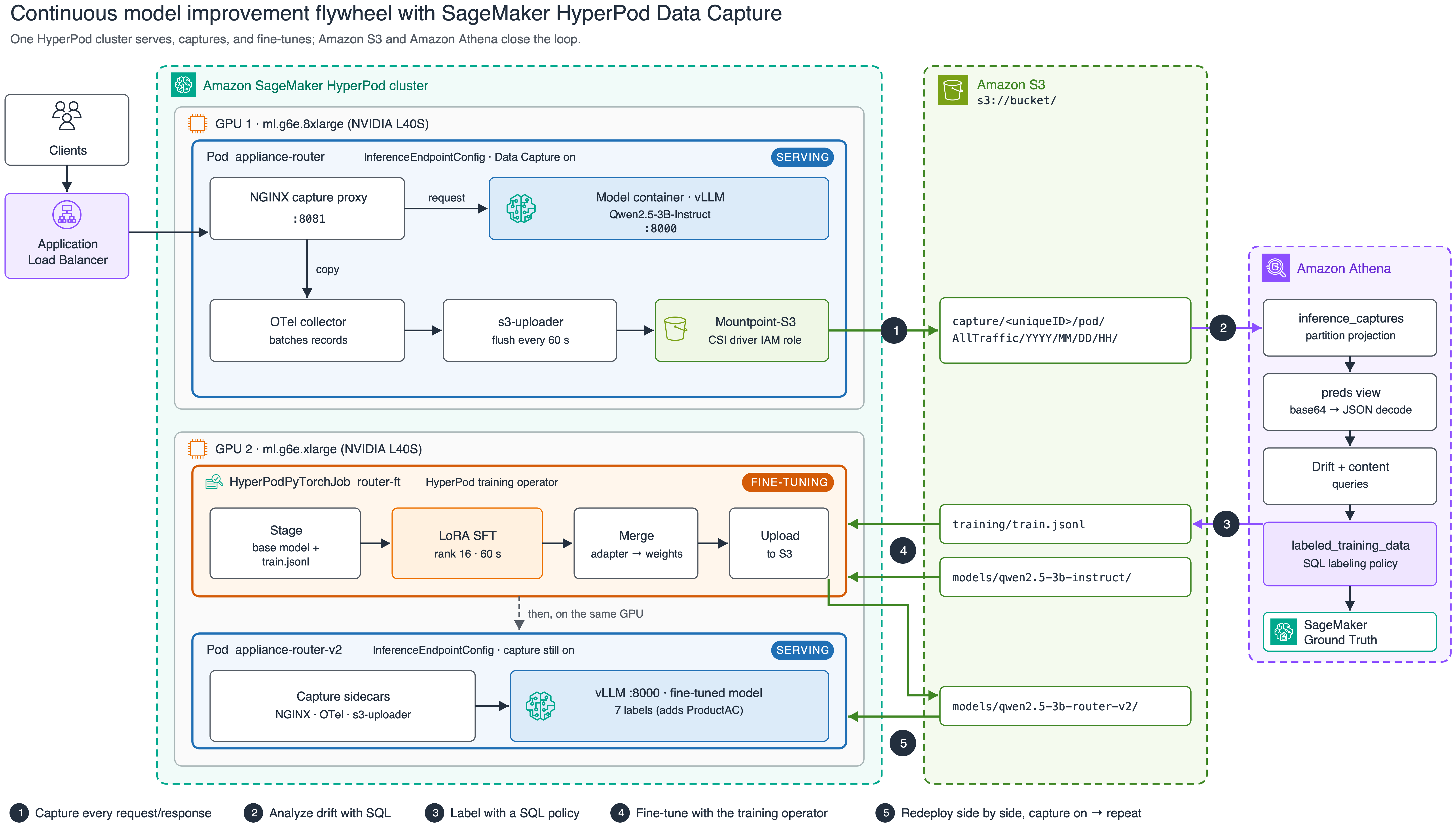
图 1:单个 SageMaker HyperPod 集群上的五步飞轮,从捕获到 Athena 分析、打标、微调,再到重新部署
推理算子会向模型 Pod 添加三个边车容器。每个经过 NGINX 代理的请求都会被复制到 OpenTelemetry 收集器,进行批处理后通过 Mountpoint-S3 卷写入 S3。Athena 会就地读取这些文件。训练算子将微调作为 HyperPodPyTorchJob 在第二块 GPU 上,新模型由第二个端点提供服务,该端点同样开启了捕获。
步骤 0:设置变量
后续每一步都会读取这些内容。请先编辑第一个代码块,然后粘贴完整内容:
# --- edit these ---
export EKS_CLUSTER_NAME="my-hyperpod-eks"
export AWS_REGION="us-east-1"
export BUCKET="amzn-s3-demo-bucket"
export SERVE_INSTANCE_TYPE="ml.g6e.8xlarge"     # node type for the first endpoint
export TRAIN_INSTANCE_TYPE="ml.g6e.xlarge"      # node type for the fine-tuning job
# --- leave as-is ---
export AWS_DEFAULT_REGION="$AWS_REGION"
export ENDPOINT_NAME="appliance-router"
export MODEL_LOCATION="models/qwen2.5-3b-instruct"
export MODEL_V2_LOCATION="models/qwen2.5-3b-router-v2"
export TRAIN_SA="flywheel"                     # service account with S3 access via EKS Pod Identity
aws eks update-kubeconfig --name "$EKS_CLUSTER_NAME" --region "$AWS_REGION"
render() { python3 -c 'import os,sys; sys.stdout.write(os.path.expandvars(sys.stdin.read()))'; }
步骤 1:将基础模型暂存到 S3
我们使用 Qwen2.5-3B-Instruct 因为它足够小,大约一分钟即可完成微调,并且能装进单块 L40S。
pip install -q huggingface_hub
python3 -c "from huggingface_hub import snapshot_download; \
  snapshot_download('Qwen/Qwen2.5-3B-Instruct', local_dir='qwen2.5-3b-instruct')"
aws s3 sync qwen2.5-3b-instruct "s3://${BUCKET}/${MODEL_LOCATION}/" --exclude ".cache/*"
步骤 2:IAM 权限
需要配置四种身份才能访问。有关策略声明,请参阅 HyperPod 上用于推理的数据捕获.
- Mountpoint-S3 CSI 驱动程序角色。 Tier 3 捕获通过 Mountpoint-S3 卷写入,驱动程序以其自身的 IAM roles for service accounts (IRSA) 角色进行身份验证,而不是以 Pod 的服务账户身份验证。它需要
s3:PutObject,s3:AbortMultipartUpload,以及s3:DeleteObject写入你的捕获存储桶,另外还需要kms:Decrypt,kms:GenerateDataKey,以及kms:DescribeKey如果缺少此项,端点会保持健康且请求成功,但不会出现任何捕获记录。kmsKeyId如果缺少此项,端点会保持健康且请求成功,但不会出现任何捕获记录。请参阅 Amazon S3 CSI 驱动程序的挂载点. - 推理算子执行角色。 它需要
s3:PutObject写入你的捕获存储桶,另外还需要kms:Decrypt以及kms:GenerateDataKey如果你设置了kmsKeyId捕获文件本身是通过 CSI 驱动程序角色写入的,因此如果没有出现任何捕获记录,请首先检查该角色。 - 训练 Pod 的服务账户(
$TRAIN_SA). 通过以下方式获得基础模型和训练数据的读取权限,以及合并模型的写入权限: EKS Pod Identity. - Athena。 对捕获前缀的读取权限,以及一个查询结果位置。
启用数据捕获
接下来的三个步骤将部署路由器并开启 Tier 3 捕获,检查 Pod 是否运行捕获边车容器,并确认记录能够到达 Amazon S3。
步骤 3:在启用 Tier 3 捕获的情况下部署模型
这就是该功能的完整内容: dataCapture.modelPod.enabled: true 代码块。其余部分都是普通的 vLLM 部署。
cat > endpoint.yaml <<'YAML'
apiVersion: inference.sagemaker.aws.amazon.com/v1
kind: InferenceEndpointConfig
metadata:
  name: ${ENDPOINT_NAME}
  namespace: default
spec:
  replicas: 1
  modelName: ${ENDPOINT_NAME}
  endpointName: ${ENDPOINT_NAME}
  instanceType: ${SERVE_INSTANCE_TYPE}
  invocationEndpoint: v1/chat/completions
  modelSourceConfig:
    modelSourceType: s3
    modelLocation: ${MODEL_LOCATION}
    s3Storage:
      bucketName: ${BUCKET}
      region: ${AWS_REGION}

  # >>> This is all you need to turn on Tier 3 data capture <<<
  dataCapture:
    s3Uri: "s3://${BUCKET}/capture/"
    modelPod:
      enabled: true
      initialSamplingPercentage: 100
      bufferConfig:
        batchSize: 50
        flushIntervalSeconds: 60
      payloadConfig:
        maxPayloadSizeKB: 1024

  worker:
    image: vllm/vllm-openai:v0.10.0
    modelInvocationPort:
      containerPort: 8000
      name: http
    modelVolumeMount:
      mountPath: /opt/ml/model
      name: model-weights
    args: ["--model", "/opt/ml/model", "--served-model-name", "${ENDPOINT_NAME}",
           "--port", "8000", "--max-model-len", "2048", "--gpu-memory-utilization", "0.90"]
    resources:
      requests: { cpu: "2", memory: 16Gi, nvidia.com/gpu: 1 }
      limits:   { nvidia.com/gpu: 1 }
YAML
render < endpoint.yaml | kubectl apply -f -
前面的 modelPod 代码块默认设置 100% 采样并同时捕获输入和输出。要调整它,请在以下位置添加这些可选字段中的任意一个: modelPod:
modelPod:
  enabled: true
  initialSamplingPercentage: 50          # capture 50% of requests (default 100)
  bufferConfig:
    batchSize: 100                       # records buffered per upload batch (default 10)
    flushIntervalSeconds: 60             # max seconds before a flush (default 60)
  payloadConfig:
    maxPayloadSizeKB: 1024               # truncate payloads larger than this (default: no limit)
  kmsKeyId: "arn:aws:kms:...:key/..."    # encrypt captures at rest
步骤 4:等待 Pod
启用捕获的 Pod 会运行 四个容器:该模型, sidecar-reverse-proxy (NGINX), otel-collector,以及 s3-uploader模型容器和 Pod 的 app 这两个标签都以 modelName.
kubectl get pods -l app=$ENDPOINT_NAME -o custom-columns=\
'NAME:.metadata.name,READY:.status.containerStatuses[*].ready,CONTAINERS:.spec.containers[*].name,NODE:.spec.nodeName'
NAME                            READY                 CONTAINERS                                                              NODE
appliance-router-849f466476-4f5v8   true,true,true,true   appliance-router,s3-uploader,sidecar-reverse-proxy,otel-collector   hyperpod-i-0f3fe2684afd6a583
在我们的运行中,Pod 在约五分钟后准备就绪, kubectl apply其中大部分时间用于下载权重。
步骤 5:发送请求并确认捕获数据写入 S3
通过端口 8081 上的捕获代理发送推理请求,然后 8081,然后在刷新间隔之后,列出捕获前缀。模型本身监听端口 8000。发送到该端口的请求会绕过代理,因此不会被捕获。
POD=$(kubectl get pod -l app=$ENDPOINT_NAME -o jsonpath='{.items[0].metadata.name}')
kubectl port-forward "pod/$POD" 18081:8081 >/dev/null 2>&1 &
sleep 5

curl -s http://localhost:18081/v1/chat/completions \
  -H 'Content-Type: application/json' \
  -d '{"model":"'"$ENDPOINT_NAME"'","messages":[{"role":"user","content":"my fridge is not cooling"}],"max_tokens":24}'

echo "Waiting for the capture buffer to flush..."; sleep 75
aws s3 ls "s3://${BUCKET}/capture/" --recursive | grep '\.jsonl$' | head
2026-09-28 15:47:14     634356 capture/20e4425092f90c7f/pod/AllTraffic/2026/09/28/15/28-15-47-12-999-ac31d31b-5156-46ad-9ccc-e8a040ab9ab2.jsonl
你会看到一个或多个 .jsonl 对象,位于 {s3Uri}/{uniqueID}/pod/{variant}/{YYYY}/{MM}/{DD}/{HH}/。 uniqueID 按端点生成。每一行都是一次推理,采用接下来展示的 SageMaker 数据捕获格式。
捕获记录格式
请求体和响应体存储在 ,正如 字段所示,因此要读回它们需要先进行 base64 解码,然后再解析 JSON:解码后, 是客户端发送的请求体, 是模型返回的响应。场景:一个支持工单路由器遇上产品发布所部署的模型是一个家电零售商的支持工单路由器。它使用 vLLM 引导式 JSON 解码,将每个工单分类为六个类别之一:、、、、、或兜底的 。引导式解码意味着它只能返回一个包含这些类别之一的有效对象,作为 encoding 字段所示,因此要读回它们需要先进行 base64 解码,然后再解析 JSON:
{
  "captureData": {
    "endpointInput":  { "observedContentType": "application/json", "mode": "INPUT",
                        "data": "eyJtb2RlbCI6ICJyb3V0ZXItZnJlc2giLCAidGVtcGVyYXR1cmUiOiAwLCAi...", "encoding": "BASE64" },
    "endpointOutput": { "observedContentType": "application/json", "mode": "OUTPUT",
                        "data": "eyJpZCI6ImNoYXRjbXBsLTctMTc5MDYxMDM2OS4wMDUtMjMxMiIsIm9iamVj...", "encoding": "BASE64" }
  },
  "eventMetadata": { "eventId": "26859f07-d60b-4683-94aa-d21e7f19e746", "inferenceTime": "2026-09-28T15:46:09Z" },
  "eventVersion": "0"
}
解码后, endpointInput.data 是客户端发送的请求体,而 endpointOutput.data 是模型返回的响应。
场景:一个支持工单路由器遇上产品发布
所部署的模型是一个家电零售商的支持工单路由器。它使用 vLLM 引导式 JSON 解码,将每个工单分类为六个类别之一: ProductFridge, ProductWasher, ProductOven, ProductDishwasher, ProductMicrowave,或兜底的“ Other。引导式解码意味着它只能返回一个带有这些标签之一的有效对象:
{"category": "ProductWasher", "confidence": 1}模型部署后,该零售商推出了自有空调产品线,即 Arctis 系列(Arctis 9K、12K、Mini 等)。路由器没有为它们设置类别。它无法说“这是新的”。它只能选择它所知道的最接近的标签。除非每个请求和响应都被记录下来,否则响应一返回,证据就消失了。
合成流量
我们生成了两个合成数据集:
- 生产流量: 900 张工单,在 15 分钟内按顺序通过捕获代理重放,使用路由器最初的六标签提示词。前 400 张出现在产品发布之前,且未提及空调。在剩余的 500 张中,Arctis 工单的占比从 15% 逐步上升到 55%。
- 评估集: 280 张已标注工单,每类 40 张,包括新增的
ProductAC它被留出 按内容:它使用的症状、句子模板和 Arctis 型号名称从未出现在流量中。
每个生产请求看起来像这样(系统提示词已简略):
{"model": "appliance-router", "temperature": 0, "max_tokens": 40,
 "messages": [{"role": "system", "content": "You are a support-ticket router for a home-appliance retailer. ... category is one of: ProductFridge, ProductWasher, ProductOven, ProductDishwasher, ProductMicrowave, Other. ..."},
              {"role": "user", "content": "Hi, our Arctis 12K blows warm air since last week. Order #66759."}],
 "guided_json": {"type": "object", "required": ["category", "confidence"],
                 "properties": {"category": {"enum": ["ProductFridge", "ProductWasher", "ProductOven",
                                                      "ProductDishwasher", "ProductMicrowave", "Other"]},
                                "confidence": {"type": "number"}}}}
要重放这些流量,请克隆随附的代码仓库,生成数据集,并通过捕获代理发送它们。 scripts/pod.sh 在模型容器内运行客户端,因此不需要负载均衡器或 DNS。客户端会打印 Athena 步骤所使用的三个时间戳: RUN_START, LAUNCH_TS (第一张发布后工单),以及 RUN_END.
git clone https://github.com/awslabs/awsome-distributed-ai.git
cd awsome-distributed-ai/examples/use-cases/sagemaker-hyperpod-data-capture-flywheel
(cd data && python3 ../scripts/gen_dataset.py)
scripts/pod.sh $ENDPOINT_NAME drive /tmp/tickets_traffic.jsonl --seconds 900
RUN_START=2026-09-28 15:52:40
  sent 100/900
...
LAUNCH_TS=2026-09-28 15:59:20
...
RUN_END=2026-09-28 16:07:40
导出你的运行所打印的三个值,并等待一个刷新间隔:
export RUN_START="2026-09-28 15:52:40" LAUNCH_TS="2026-09-28 15:59:20" RUN_END="2026-09-28 16:07:40"
sleep 75    # one flush interval
揭示 Amazon Athena 中的问题
发布之后,离线基准测试看起来仍然没有变化,因为它们被冻结在过去。这种变化只在采集到的生产流量中才能看到。本节展示数据科学家如何在不配置任何基础设施的情况下,用 Athena 发现它。
第 6 步:设置变量并配置 Athena 辅助函数
export ATHENA_DB="flywheel_demo"
export ATHENA_OUTPUT="s3://${BUCKET}/athena-results/"
# Each endpoint writes under its own uniqueID. Pick the prefix whose captured requests name this
# endpoint, not whichever prefix sorts first (the Step 15 endpoint adds a second one).
for id in $(aws s3 ls "s3://${BUCKET}/capture/" | awk '/PRE/{print $2}'); do
  key=$(aws s3 ls "s3://${BUCKET}/capture/${id}pod/AllTraffic/" --recursive | awk '/\.jsonl$/{print $4; exit}')
  [ -n "$key" ] || continue
  model=$(aws s3 cp "s3://${BUCKET}/${key}" - 2>/dev/null | head -n 1 | python3 -c 'import sys, json, base64; r = json.loads(sys.stdin.readline()); print(json.loads(base64.b64decode(r["captureData"]["endpointInput"]["data"]))["model"])')
  if [ "$model" = "$ENDPOINT_NAME" ]; then export CAPTURE_LOCATION="s3://${BUCKET}/capture/${id}pod/AllTraffic/"; break; fi
done
echo "$CAPTURE_LOCATION"     # s3://<bucket>/capture/<uniqueID>/pod/AllTraffic/

# run_athena "<SQL>": runs one statement, prints tab-separated rows, and sets LAST_QID
run_athena() {
  local qid st
  qid=$(aws athena start-query-execution --query-string "$1" \
        --query-execution-context "Database=$ATHENA_DB" \
        --result-configuration "OutputLocation=$ATHENA_OUTPUT" \
        --output text --query 'QueryExecutionId') || return 1
  while :; do
    st=$(aws athena get-query-execution --query-execution-id "$qid" \
         --output text --query 'QueryExecution.Status.State')
    case "$st" in
      SUCCEEDED) break ;;
      FAILED|CANCELLED) aws athena get-query-execution --query-execution-id "$qid" \
          --output text --query 'QueryExecution.Status.StateChangeReason' >&2; return 1 ;;
    esac
    sleep 2
  done
  LAST_QID=$qid
  aws athena get-query-results --query-execution-id "$qid" \
    --output text --query 'ResultSet.Rows[*].Data[*].VarCharValue'
}
run_athena "CREATE DATABASE IF NOT EXISTS ${ATHENA_DB}"
第 7 步:向 Athena 声明捕获数据(两层)
第一层是信封。外部表描述每条记录的外层 JSON,而分区投影则 year/month/day/hour 将每小时 S3 前缀映射到分区,无需爬虫或 ADD PARTITION。 data 这些字段被声明为普通字符串,因为它们是 base64 文本。
run_athena "
CREATE EXTERNAL TABLE IF NOT EXISTS inference_captures (
  captureData struct<
    endpointInput:  struct<observedContentType: string, mode: string, data: string, encoding: string>,
    endpointOutput: struct<observedContentType: string, mode: string, data: string, encoding: string>
  >,
  eventMetadata struct<eventId: string, inferenceTime: string>,
  eventVersion string
)
PARTITIONED BY (year string, month string, day string, hour string)
ROW FORMAT SERDE 'org.openx.data.jsonserde.JsonSerDe'
LOCATION '${CAPTURE_LOCATION}'
TBLPROPERTIES (
  'projection.enabled'='true',
  'projection.year.type'='integer',  'projection.year.range'='2026,2035',
  'projection.month.type'='integer', 'projection.month.range'='1,12', 'projection.month.digits'='2',
  'projection.day.type'='integer',   'projection.day.range'='1,31',   'projection.day.digits'='2',
  'projection.hour.type'='integer',  'projection.hour.range'='0,23',  'projection.hour.digits'='2',
  'storage.location.template'='${CAPTURE_LOCATION}\${year}/\${month}/\${day}/\${hour}/'
)"
第二层是一个视图,它对每条记录只解码一次。 from_utf8(from_base64(...)) 会将这些负载转换回 JSON。如果没有它,每次提取都会返回 NULL。工单就是用户消息(messages[1],因为 messages[0] 是系统提示词)。模型的回答是响应 JSON 中的一个 JSON 字符串,因此需要再进行一次提取。
run_athena "
CREATE OR REPLACE VIEW preds AS
WITH decoded AS (
  SELECT CAST(from_iso8601_timestamp(eventMetadata.inferenceTime) AS timestamp) AS ts,
         from_utf8(from_base64(captureData.endpointInput.data))  AS req,
         from_utf8(from_base64(captureData.endpointOutput.data)) AS resp
  FROM inference_captures
  WHERE year = '${RUN_START:0:4}' AND month = '${RUN_START:5:2}' AND day = '${RUN_START:8:2}'
)
SELECT ts,
       json_extract_scalar(req, '\$.messages[1].content') AS ticket_text,
       json_extract_scalar(json_extract_scalar(resp, '\$.choices[0].message.content'), '\$.category') AS predicted_category,
       CAST(json_extract_scalar(json_extract_scalar(resp, '\$.choices[0].message.content'), '\$.confidence') AS double) AS confidence
FROM decoded
WHERE ts >= timestamp '${RUN_START}' AND ts < timestamp '${RUN_END}'
"
run_athena "SELECT count(*) AS n, count_if(predicted_category IS NULL) AS unparsed FROM preds"
n   unparsed
900 0
关于该视图的两点说明:
- 始终按分区进行过滤。 Athena 读取原始 JSON,因此不带分区过滤条件的查询会扫描你曾经捕获的每一个对象。该视图会过滤到某一天,而时间界限会将其限制在我们的流量运行范围内:同一前缀下还保存着第 5 步的请求。
messages[1]假设一条系统消息后跟一条用户消息。 捕获的流量就是客户端实际发送的内容,因此请针对多轮或少样本请求调整提取逻辑。
第 8 步:类别构成是否在变化?
run_athena "
SELECT date_trunc('minute', ts) AS minute, count(*) AS tickets,
       count_if(predicted_category = 'Other') AS other,
       round(100.0 * count_if(predicted_category = 'Other') / count(*), 1) AS other_pct
FROM preds GROUP BY 1 ORDER BY 1"
minute                   tickets  other  other_pct
2026-09-28 15:52:00.000       20      0        0.0
2026-09-28 15:53:00.000       60      3        5.0
2026-09-28 15:54:00.000       60      4        6.7
2026-09-28 15:55:00.000       60      4        6.7
2026-09-28 15:56:00.000       60      2        3.3
2026-09-28 15:57:00.000       60      1        1.7
2026-09-28 15:58:00.000       60      3        5.0
2026-09-28 15:59:00.000       60      9       15.0
2026-09-28 16:00:00.000       60     17       28.3
2026-09-28 16:01:00.000       60     14       23.3
2026-09-28 16:02:00.000       60     19       31.7
2026-09-28 16:03:00.000       60     21       35.0
2026-09-28 16:04:00.000       60     20       33.3
2026-09-28 16:05:00.000       60     32       53.3
2026-09-28 16:06:00.000       60     28       46.7
2026-09-28 16:07:00.000       40     26       65.0
(输出以制表符分隔。为便于阅读,我们在此进行了对齐。我们的运行将“数周”压缩为 15 分钟。在生产环境中,请按 date_trunc('day', ts) 或 'week' (改为)
下图绘制了每分钟路由到 Other 为柱状图,累计份额为折线,并标出发布时刻。
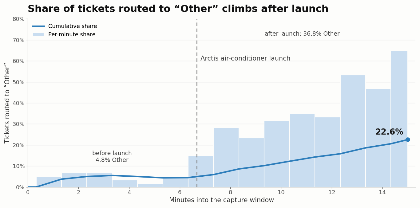
图 2:Arctis 发布前后,每分钟及累计路由到 Other 的工单占比
在发布之前, Other 每分钟保持在 7% 以下。在发布的那一分钟,它跃升至 15%,并持续攀升,在最后三分钟达到 47–65%。图表中的累计曲线只达到 22.6%,因为它把发布后的工单与发布前的所有流量一起做了平均。这就是为什么你会把每分钟速率、而不是累计份额,作为告警的触发依据。
按发布时刻拆分,整体类别构成如下:
run_athena "
SELECT IF(ts < timestamp '${LAUNCH_TS}', '1-before launch', '2-after launch') AS period,
       predicted_category, count(*) AS n
FROM preds GROUP BY 1, 2 ORDER BY 1, 3 DESC"
period           predicted_category    n
1-before launch  ProductFridge        91
1-before launch  ProductWasher        83
1-before launch  ProductDishwasher    74
1-before launch  ProductOven          74
1-before launch  ProductMicrowave     59
1-before launch  Other                19
2-after launch   Other               184
2-after launch   ProductFridge        84
2-after launch   ProductOven          66
2-after launch   ProductDishwasher    64
2-after launch   ProductWasher        58
2-after launch   ProductMicrowave     44
Other 从 4.8% 发布前工单占比(400 张中的 19 张)到 36.8% 之后(500 张中的 184 张),并成为最大的类别。
第 9 步:Other 桶里有什么?
run_athena "
SELECT word, count(*) AS freq
FROM preds CROSS JOIN UNNEST(regexp_extract_all(lower(ticket_text), '[a-z0-9-]{4,}')) AS t(word)
WHERE predicted_category = 'Other'
  AND word NOT IN ('this','that','with','from','have','since','week','help','need','again','time',
                   'month','second','take','look','someone','order','last','after','when','onto')
GROUP BY 1 ORDER BY 2 DESC, 1 LIMIT 10"
word      freq
arctis     141
unit        40
mini        33
cooling     30
link        30
lost        30
loudly      30
rattles     30
wi-fi       30
blows       28
这个 Other 桶里并不是一堆互不相关的工单。它被一个产品名称主导, arctis以及制冷电器的词汇,这指向了一个路由器没有对应标签的新类别。
第 10 步:它有多大,模型的置信度是否会标记它?
在整个流量流中搜索新产品,而不仅仅是 Other 桶:
run_athena "
SELECT IF(ts < timestamp '${LAUNCH_TS}', '1-before launch', '2-after launch') AS period,
       predicted_category, count(*) AS n
FROM preds WHERE regexp_like(lower(ticket_text), 'arctis|air condition')
GROUP BY 1, 2 ORDER BY 1, 3 DESC"
period          predicted_category    n
2-after launch  Other               164
2-after launch  ProductFridge        14
共有 178 张空调工单,占全部流量的 19.8%。它们没有一张出现在发布之前。 它们分为两组:
- 164 张进入了
Other. 在六标签模式下,这就是 正确 答案:Other正是为这种情况而存在。路由器并没有坏。分类体系缺少一个类别,因此这些工单进入了通用队列,而不是进入支持该产品的团队。 - 14 张进入了
ProductFridge. 这些是真正的错误路由:冰箱团队现在收到的是空调工单。
现在测试模型对这些已知错误路由的置信度:
run_athena "
SELECT predicted_category, confidence, count(*) AS n FROM preds
WHERE regexp_like(lower(ticket_text), 'arctis|air condition')
GROUP BY 1, 2 ORDER BY 1, 2 DESC"
predicted_category  confidence    n
Other                      1.0  157
Other                      0.9    7
ProductFridge             0.95    1
ProductFridge              0.9    9
ProductFridge              0.8    2
ProductFridge              0.7    1
ProductFridge              0.0    1
在14张被错误路由的工单中,有10张报告的置信度为0.9或更高。诸如“保留预测结果,只要其 confidence >= 0.9”本可以保留 71% 的已知错误标签。这是因为 confidence 是我们要求模型写出的字段,而不是经过校准的概率。如果你需要真正的不确定性信号,请从 vLLM 请求 token logprobs 从 vLLM 中获取,并读取类别 token 处的概率,而不是模型的自报结果。要为额外的负载大小预留预算,因为 logprobs 都会随每个响应一并捕获。
从诊断到带标签的训练数据
数据科学家不会手动标注数百张工单。相反,他们会把 Athena 的发现写成一个 打标策略:一个为每条捕获记录分配修正后标签的 SQL 视图。我们将被错误路由的空调工单重新标记为新类别。
第 11 步:打标策略
run_athena "
CREATE OR REPLACE VIEW labeled_training_data AS
WITH t AS (SELECT ticket_text, predicted_category, lower(ticket_text) AS txt FROM preds)
SELECT ticket_text, predicted_category,
  CASE
    -- 1. The new class, identified by keyword evidence, not by what the model predicted
    WHEN regexp_like(txt, '\\barctis\\b|air condition|\\bac unit\\b|mini split')
     AND NOT regexp_like(txt, 'fridge|refrigerat|freezer|washer|\\boven\\b|\\brange\\b|dishwasher|microwave')
      THEN 'ProductAC'
    -- 2. Keep the production decision when nothing hints at the new product
    WHEN NOT regexp_like(txt, '\\barctis\\b|air condition|\\bac\\b|mini split')
      THEN predicted_category
    -- 3. Mixed signals: send to human review (Amazon SageMaker Ground Truth)
    ELSE NULL
  END AS corrected_category
FROM t"双反斜杠(\\b)是在双引号字符串内部进行 shell 转义。Athena 会收到 \b,一个正则表达式单词边界。
检查该策略产生了什么:
run_athena "
SELECT coalesce(corrected_category, '(human review)') AS label, count(*) AS n,
       count(DISTINCT ticket_text) AS distinct_texts,
       count_if(corrected_category <> predicted_category) AS relabeled
FROM labeled_training_data GROUP BY 1 ORDER BY 2 DESC"
label               n    distinct_texts  relabeled
ProductAC         178               114        178
ProductFridge     161               110          0
ProductWasher     141                96          0
ProductOven       140                97          0
ProductDishwasher 138                95          0
ProductMicrowave  103                82          0
Other              39                 8          0
这个启发式方法之所以有效,是因为新类别界限清晰(可通过关键词识别)。对于模糊工单或类别重叠的情况,NULL 行会被路由到 Ground Truth 进行人工标注。
第 12 步:构建训练文件
导出带标签的视图并将其转换为聊天格式的 JSONL。允许的类别集合现在包括 ProductAC,即重新部署后客户端将发送的同一个七标签提示词。将其保存为 build_training_file.py:
cat > build_training_file.py <<'PY'
import csv, json, sys
CATS = ["ProductFridge", "ProductWasher", "ProductOven", "ProductDishwasher", "ProductMicrowave", "ProductAC", "Other"]
PROMPT = ("You are a support-ticket router for a home-appliance retailer. Route each ticket to the product it "
          'concerns. Respond with ONLY a JSON object {"category": "...", "confidence": <0-1>} where category is '
          "one of: " + ", ".join(CATS) + '. Use "Other" if the ticket does not clearly concern one of these products.')
n = 0
with open(sys.argv[1], newline="") as fin, open(sys.argv[2], "w") as fout:
    for row in csv.DictReader(fin):
        fout.write(json.dumps({"messages": [
            {"role": "system", "content": PROMPT},
            {"role": "user", "content": row["ticket_text"]},
            {"role": "assistant", "content": json.dumps({"category": row["corrected_category"], "confidence": 1.0})},
        ]}) + "\n"); n += 1
print(f"wrote {n} training examples -> {sys.argv[2]}")
PY

run_athena "SELECT ticket_text, corrected_category FROM labeled_training_data
            WHERE corrected_category IS NOT NULL" > /dev/null
aws s3 cp "${ATHENA_OUTPUT}${LAST_QID}.csv" labeled.csv --only-show-errors   # Athena's own CSV: header + proper quoting
python3 build_training_file.py labeled.csv train.jsonl
aws s3 cp train.jsonl "s3://${BUCKET}/training/train.jsonl"
wrote 900 training examples -> train.jsonl
使用 HyperPod 训练算子对采集到的数据进行微调
我们在为模型提供服务的同一集群上进行微调,使用 HyperPod 训练算子并占用第二块 GPU。第一个端点全程保持服务。
第 13 步:训练脚本
该脚本从 S3 下载基础模型和训练数据,并训练一个低秩适配(LoRA)适配器。损失仅在助手回合上计算,因此模型学习生成标签,而不是重复提示词。随后脚本将适配器合并回基础权重,使 vLLM 能够原样提供结果,并将合并后的模型上传到 S3。该作业通过 ConfigMap 将脚本挂载到训练 Pod 中。
cat > train.py <<'PY'
import os, boto3, torch
from datasets import load_dataset
from peft import LoraConfig, get_peft_model
from transformers import AutoModelForCausalLM, AutoTokenizer, Trainer, TrainingArguments

s3 = boto3.client("s3")
def split(uri): b, _, k = uri[5:].partition("/"); return b, k

# 1. Stage base model + training data from S3
bucket, prefix = split(os.environ["BASE_MODEL_S3"])
for page in s3.get_paginator("list_objects_v2").paginate(Bucket=bucket, Prefix=prefix):
    for o in page.get("Contents", []):
        dst = os.path.join("/work/base", os.path.relpath(o["Key"], prefix))
        os.makedirs(os.path.dirname(dst), exist_ok=True); s3.download_file(bucket, o["Key"], dst)
s3.download_file(*split(os.environ["TRAIN_FILE_S3"]), "/work/train.jsonl")
print("[stage] base model and training data downloaded", flush=True)

# 2. LoRA SFT, loss only on the assistant turn (the label), not the prompt
tok = AutoTokenizer.from_pretrained("/work/base")
def encode(ex):
    full = tok.apply_chat_template(ex["messages"], tokenize=False)
    prompt = tok.apply_chat_template(ex["messages"][:-1], tokenize=False, add_generation_prompt=True)
    ids = tok(full, add_special_tokens=False)["input_ids"]
    n = len(tok(prompt, add_special_tokens=False)["input_ids"])
    return {"input_ids": ids, "labels": [-100] * n + ids[n:]}
ds = load_dataset("json", data_files="/work/train.jsonl", split="train")
print(f"[data] {len(ds)} examples", flush=True)
ds = ds.map(encode, remove_columns=ds.column_names)

def collate(batch):
    m = max(len(b["input_ids"]) for b in batch)
    pad = lambda xs, v: [x + [v] * (m - len(x)) for x in xs]
    return {"input_ids": torch.tensor(pad([b["input_ids"] for b in batch], tok.pad_token_id)),
            "labels": torch.tensor(pad([b["labels"] for b in batch], -100)),
            "attention_mask": torch.tensor(pad([[1] * len(b["input_ids"]) for b in batch], 0))}

model = AutoModelForCausalLM.from_pretrained("/work/base", torch_dtype=torch.bfloat16, device_map="cuda:0")
model = get_peft_model(model, LoraConfig(r=16, lora_alpha=32, lora_dropout=0.05, task_type="CAUSAL_LM",
    target_modules=["q_proj", "k_proj", "v_proj", "o_proj", "gate_proj", "up_proj", "down_proj"]))
model.print_trainable_parameters()
Trainer(model=model, train_dataset=ds, data_collator=collate, args=TrainingArguments(
    output_dir="/tmp/ckpt", num_train_epochs=float(os.getenv("EPOCHS", "2")), learning_rate=1e-4,
    per_device_train_batch_size=8, bf16=True, logging_steps=10, save_strategy="no", report_to=[],
    warmup_ratio=0.1, lr_scheduler_type="cosine")).train()

# 3. Merge the adapter into the base weights (a plain model vLLM can serve) and upload it
model.merge_and_unload().save_pretrained("/work/out", safe_serialization=True)
tok.save_pretrained("/work/out")
bucket, prefix = split(os.environ["OUTPUT_S3"])
for f in os.listdir("/work/out"):
    s3.upload_file(os.path.join("/work/out", f), bucket, f"{prefix.rstrip('/')}/{f}")
print(f"[done] merged model uploaded to {os.environ['OUTPUT_S3']}", flush=True)
PY
kubectl create configmap router-train --from-file=train.py
第 14 步:提交 HyperPodPyTorchJob
cat > finetune-job.yaml <<'YAML'
apiVersion: sagemaker.amazonaws.com/v1
kind: HyperPodPyTorchJob
metadata:
  name: router-ft
  namespace: default
spec:
  nprocPerNode: "1"
  runPolicy:
    jobMaxRetryCount: 2
    cleanPodPolicy: All              # release the GPU as soon as the job finishes
    logMonitoringConfiguration:      # restart a job that never starts, or goes quiet mid-run
      - name: JobStart
        logPattern: '.*loss.*'
        expectedStartCutOffInSeconds: 1200
      - name: JobHangingDetection
        logPattern: '.*loss.*'
        expectedRecurringFrequencyInSeconds: 600
  replicaSpecs:
    - name: pod
      replicas: 1
      template:
        metadata:
          labels: { app: router-ft }
        spec:
          serviceAccountName: ${TRAIN_SA}        # EKS Pod Identity -> S3 read/write
          nodeSelector:
            node.kubernetes.io/instance-type: ${TRAIN_INSTANCE_TYPE}
          restartPolicy: Always                  # required by the operator; retries live in runPolicy
          containers:
            - name: pytorch
              image: vllm/vllm-openai:v0.10.0    # already has torch + transformers + boto3
              command: ["bash", "-c"]
              args:
                - pip install -q peft==0.14.0 datasets==3.2.0 hyperpod-elastic-agent==1.1.3 &&
                  hyperpodrun --nnodes=1 --nproc_per_node=1 /scripts/train.py
              env:
                - { name: BASE_MODEL_S3, value: "s3://${BUCKET}/${MODEL_LOCATION}/" }
                - { name: TRAIN_FILE_S3, value: "s3://${BUCKET}/training/train.jsonl" }
                - { name: OUTPUT_S3,     value: "s3://${BUCKET}/${MODEL_V2_LOCATION}/" }
              resources:
                requests: { cpu: "2", memory: 24Gi, nvidia.com/gpu: 1 }
                limits:   { nvidia.com/gpu: 1 }
              volumeMounts:
                - { name: scripts, mountPath: /scripts }
                - { name: work,    mountPath: /work }
                - { name: shm,     mountPath: /dev/shm }
          volumes:
            - { name: scripts, configMap: { name: router-train } }
            - { name: work,    emptyDir: {} }
            - { name: shm,     emptyDir: { medium: Memory, sizeLimit: 8Gi } }
YAML
render < finetune-job.yaml | kubectl apply -f -
kubectl logs -l app=router-ft -flogMonitoringConfiguration是训练算子区别于其他算子的特征。 如果未出现loss如果启动后 20 分钟内出现该行,或者运行中途日志静默 10 分钟而进程仍然存活,运维人员会重启作业,而不是让它白白消耗 GPU 时长。- 该作业在启动时会安装三个 Python 包。 训练节点需要具备出站互联网访问能力(例如通过 NAT 网关),从 Docker Hub 拉取镜像也同样需要。
vllm/vllm-openai镜像从 Docker Hub 拉取。在没有互联网出口的集群上,将软件包烘焙到 Amazon Elastic Container Registry(Amazon ECR)中的自定义镜像里,并去掉pip install.
作业日志摘录:
{'loss': 0.2484, 'grad_norm': 3.387, 'learning_rate': 3.91e-05, 'epoch': 0.09}
{'loss': 0.018, 'grad_norm': 0.0037, 'learning_rate': 8.26e-05, 'epoch': 0.18}
...
{'loss': 0.0, 'grad_norm': 0.000105, 'learning_rate': 2.93e-07, 'epoch': 1.95}
{'train_runtime': 59.68, 'train_samples_per_second': 30.16, 'train_loss': 0.0123, 'epoch': 2.0}
[done] merged model uploaded to s3://amzn-s3-demo-bucket/models/qwen2.5-3b-router-v2/
[HyperPodElasticAgent] ... Transitioned from AgentState.RUNNING to AgentState.COMPLETED
kubectl get hyperpodpytorchjob router-ft -o jsonpath='{range .status.conditions[*]}=  {end}'
Created=True  Completed=True
训练耗时 60 秒 在单块 L40S 上。rank 16 的 LoRA 训练约 2990 万个参数,不到这个 31 亿参数模型的 1%。平均训练损失为 0.0123,单步损失在第一个 epoch 内就降到了 0.0,这说明模型很容易就记住了 900 个模板化示例。在真实数据上,应留出验证集并提前停止。这里我们依赖留出的评估集。
第 15 步:将微调后的模型并排部署,同时保持采集开启
不要直接编辑正在运行的端点,而是将新模型部署为一个 第二个端点 从同一个清单中,部署到训练作业刚刚释放的 GPU 上。第一个端点会持续提供服务,直到你将客户端切换过去,因此重新部署不会造成停机,而回滚只需将客户端重新指向第一个端点。
export ENDPOINT_NAME="appliance-router-v2" MODEL_LOCATION="$MODEL_V2_LOCATION" SERVE_INSTANCE_TYPE="$TRAIN_INSTANCE_TYPE"
render < endpoint.yaml | kubectl apply -f -
kubectl get pods -l app=$ENDPOINT_NAME -o custom-columns='NAME:.metadata.name,READY:.status.containerStatuses[*].ready,NODE:.spec.nodeName'
NAME                                  READY                 NODE
appliance-router-v2-c96594c5-fhs2x    true,true,true,true   hyperpod-i-0e0b756209b5e497a
新端点将采集数据写入其自身的 uniqueID。因为 ENDPOINT_NAME 现在为 appliance-router-v2重新运行 CAPTURE_LOCATION 第 6 步的查询会找到该前缀,因此你可以让第二个 Athena 表指向它,以进行下一轮分析。迁移客户端时,请在同一版本中更新端点、标签集和 guided-JSON 枚举。
衡量提升效果
我们用同样的 280 张留出工单对微调后的端点进行了测试:
overall 280/280 = 100.00%
  ProductFridge      40/40
  ProductWasher      40/40
  ProductOven        40/40
  ProductDishwasher  40/40
  ProductMicrowave   40/40
  ProductAC          40/40
Other 40/40| 指标 | 微调前(发布时) | 微调后 |
| 留出准确率(280) | 235 (83.9%) | 280 (100%) |
ProductAC (40) |
0/40 — 全部路由到 Other |
40/40 |
Other (40) |
35/40 | 40/40 |
| 五个既有产品类别(200) | 200/200 | 200/200 |
| 手写探针(24 条,下文将说明) | 16/24 | 20/24 |
微调让路由器学会了新类别,并且对五个既有类别没有造成任何性能回退。它还修复了五个 Other 在发布之前就已存在、并由已发布的路由器发送到 ProductFridge.
由于我们的评估集与训练数据来自同一个生成器,我们还手工编写了 24 张探针工单,采用生成器从不产生的风格。微调后的模型得分为 20/24:
  MISS ProductFridge -> ProductAC: The cooling fan in my fridge is squealing.
  MISS Other -> ProductAC: When will the Arctis 12K be back in stock?
  MISS Other -> ProductAC: Can I get a quote to install central air in my house?
  MISS Other -> ProductAC: Do you price match the Arctis at other stores?
overall 20/24 = 83.33%
它能正确路由全部八个空调探针,但学到了两个捷径:“cooling”意味着空调,而任何提到 Arctis 的内容都意味着 ProductAC,包括库存和价格匹配问题。两者都来自训练数据:标注策略把每张 Arctis 工单都发送到 ProductAC,而且采集到的流量中不包含任何售前问题。在新端点上开启采集后,这些工单正是下一轮采集所要收集的内容。
采集会带来多少延迟?
我们直接测量了这一点:同样的 400 个路由请求,从 Pod 内部分别发送到端口 8000(不采集)或端口 8081(经过采集代理)。我们以 8 个并发请求运行了三轮,另外还运行了一轮串行请求:
| 路径 | 并发 | p99吞吐量直接发送到 vLLM(8000),不采集8200.7 ms249.4 ms39.1 req/s经过采集代理(8081)8200.0 ms249.8 ms39.1 req/s直接发送到 vLLM(8000),不采集1164.4 ms206.9 ms6.0 req/s经过采集代理(8081)1164.4 ms207.0 ms6.0 req/s并发数为 8 的行是三轮的平均值。轮次之间的波动(p50 处为 ±1 ms)大于两条路径之间的差异。采集数据的其他用途推理数据写入 S3 后,同一批记录可服务于许多工作流:改进 | 采集会增加多少延迟?我们直接进行了测量:同样的 400 个路由请求,从 Pod 内部发送到端口 8000(不采集)或端口 8081(经过采集代理)。我们以 8 个并发请求运行了三轮,另外还运行了一轮串行请求:路径并发p50 | 吞吐量 |
| 直接发送到 vLLM(8000),不采集 | 8 | 200.7 毫秒 | 249.4 毫秒 | 39.1 请求/秒 |
| 经过采集代理(8081) | 8 | 200.0 毫秒 | 249.8 毫秒 | 39.1 请求/秒 |
| 直接发送到 vLLM(8000),不采集 | 1 | 164.4 毫秒 | 206.9 毫秒 | 6.0 请求/秒 |
| 经过采集代理(8081) | 1 | 164.4 ms | 207.0 毫秒 | 6.0 请求/秒 |
并发数为 8 的行是三轮的平均值。轮次之间的波动(p50 处为 ±1 ms)大于两条路径之间的差异。
采集数据的其他用途
推理数据写入 S3 后,同一批记录可服务于许多工作流:
- 改进模型: 使用监督微调(此处所示)、将大模型的输出蒸馏到较小的模型,或构建偏好对以进行直接偏好优化(DPO)。
- 理解模型: 运行 Athena 分析(此处所示),基于真实提示构建黄金回归集,设置漂移告警,发现新兴意图,并检测格式错误的输出和拒绝响应。
- 运营与治理: 将模糊样本路由到 Ground Truth 进行标注,保留审计轨迹(推荐 Tier 1),重放事件背后的精确输入,并分析流量和负载以进行成本归因。
成本考量
| 层级 | 近似成本影响 |
| Tier 1(SageMaker 端点) | 由 SageMaker 在端点处采集。你需要为负载数据支付 S3 存储和请求费用 |
| Tier 2(ALB 访问日志) | 仅日志文件的 S3 存储 |
| Tier 3(模型 Pod) | 三个边车请求 每个 Pod 总计 250m CPU + 640 MiB(NGINX 代理 100m/128Mi、OTel collector 100m/256Mi、50m/256Mi),外加负载数据的 S3 存储和请求费用 每个 Pod 总计(NGINX 代理 100m/128Mi、OTel collector 100m/256Mi、 s3-uploader 50m/256Mi),外加负载数据的 S3 存储和请求费用 |
有两项成本会随使用量增长:
- 我们的记录平均每条约 2.3 KB(9.0 MB 中共 3,955 条记录)。提示和响应越长,成本按比例越高。上传器在每个刷新间隔内为每个 Pod 写入一个对象,在 60 秒间隔下每个 Pod 每天约 1,440 次 PUT。Athena 按扫描的数据量计费,因此务必按分区列进行过滤,并使用 (CTAS) 查询将原始 JSON 转换为 Parquet,以便重复分析。有关当前价格,请参阅 Amazon S3 定价和 Amazon Athena 定价。清理为避免产生不必要的费用,请清理 我们的记录平均每条约 2.3 KB(9.0 MB 中共 3,955 条记录)。提示和响应越长,成本按比例越高。上传器在每个刷新间隔内为每个 Pod 写入一个对象,在 60 秒间隔下每个 Pod 每天约 1,440 次 PUT。
- Athena 按扫描的数据量计费,因此务必按分区列进行过滤,并使用
CREATE TABLE AS SELECT(CTAS)查询以进行重复分析。
有关当前价格,请参阅 Amazon S3 定价 以及 Amazon Athena 定价.
清理
为避免产生不必要的费用,请清理本演练中创建的资源:
kubectl delete inferenceendpointconfig appliance-router appliance-router-v2
kubectl delete hyperpodpytorchjob router-ft
kubectl delete configmap router-train
run_athena "DROP VIEW IF EXISTS labeled_training_data"; run_athena "DROP VIEW IF EXISTS preds"
run_athena "DROP TABLE IF EXISTS inference_captures"; run_athena "DROP DATABASE IF EXISTS ${ATHENA_DB}"
aws s3 rm "s3://${BUCKET}/capture/" --recursive
aws s3 rm "s3://${BUCKET}/athena-results/" --recursive
aws s3 rm "s3://${BUCKET}/training/" --recursive
aws s3 rm "s3://${BUCKET}/${MODEL_V2_LOCATION}/" --recursive
结论
在本文中,我们展示了如何使用 SageMaker HyperPod Data Capture 记录实时推理数据并将其转化为训练数据。由于数据捕获可在三个独立层级使用,您可以:
- 采集真实世界的训练数据,且对服务延迟没有可测量的影响。
- 借助 Amazon Athena 大规模查询推理模式,无需管理任何基础设施。
- 将 Athena 诊断转化为可复现的 SQL 打标策略。
- 基于采集到的生产数据进行微调,并衡量微调前后确凿的提升效果。
- 将其余循环与 HyperPod 训练算子和 SageMaker Ground Truth 集成。
我们在一个家电客服路由器上完整运行了一轮循环。捕获的流量揭示了一个新产品盲点,而一条 SQL 打标策略将这些捕获数据转化为训练数据。使用 HyperPod 训练算子进行的 60 秒 LoRA 微调,运行在服务于该模型的同一集群上。它使新类别从 0% 提升到完全召回,且对任何现有类别都没有出现回退。这些训练数据在模型部署之前都不存在。
Data Capture 现已在配备推理算子的 SageMaker HyperPod 集群上可用。要开始使用,请将 dataCapture 部分添加到你的 InferenceEndpointConfig 或 JumpStartModel 资源并部署。要在同一集群上闭环,请添加 amazon-sagemaker-hyperpod-training-operator EKS 附加组件。本演练的完整代码位于 配套的 GitHub 仓库.
更多信息,请参阅 SageMaker HyperPod 推理文档 以及 HyperPod 训练算子文档.